Curve Stablecoin - Deep dive

Introduction

Statemind recently finished an audit of Curve stablecoin and decided that a protocol this intricate and complex deserves another good article describing its inner workings. The article is based on the original work by Paco with added insights from our auditing team.

Curve Stablecoin Interpretation

Curve Stablecoin is a new generation stablecoin protocol designed by the Curve team. Compared to traditional stablecoin protocols or lending protocols such as MakerDAO, Liquity, Compound, etc., the main improvement of Curve Stablecoin lies in its built-in AMM (Automated Market Maker), which more efficiently resolves liquidation issues, thereby greatly reducing the risk of bad debt. At the same time, this AMM can help smooth the selling of assets, thereby reducing the impact of market volatility.

Traditional lending/stablecoin protocols

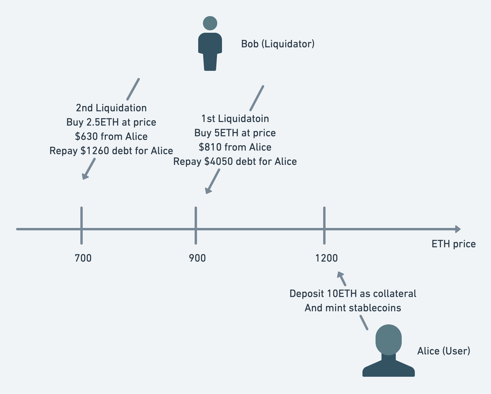
In the illustration, user Alice collateralizes 10 ETH at an ETH price of $1200 and mints stablecoins. Let's assume Alice's liquidation line is at $900. When the price reaches $900, Bob, as a liquidator, buys 5 ETH (liquidating half of the assets) from Alice's account for $810 (a 90% discount) and helps Alice repay a debt of $4050. After the liquidation, Alice has 5 ETH left in her collateral, her debt is reduced by $4050, and her margin rate returns to a healthy level. If the price continues to fall to $700, Alice will face a second liquidation. In this liquidation, Bob buys 2.5 ETH from Alice's account for $630, helping Alice repay a debt of $1260. If the price continues to fall, Alice will continue to be liquidated until all her assets are liquidated.

Drawback

This liquidation process has the following problems:

1. When the user's margin rate is insufficient, the protocol needs to liquidate a portion of the user's assets. If the user has too many assets, this means a large number of assets will need to be liquidated at once.

2. Liquidators often use flash loans to improve capital utilization. After the liquidation, they need to immediately sell the liquidated assets to repay the flash loan, which can create significant selling pressure in the spot market. When there's a large position of assets awaiting liquidation, the spot market prices will likely plummet.

3. If asset prices continue to fall and liquidation cannot be completed in time, the protocol faces the risk of bad debt.

4. To ensure liquidators are sufficiently incentivized, users' assets are sold at a low price, leading to significant losses for the users with each liquidation.

5. Once liquidation occurs, it results in irreversible losses for the user. Even if the price of the collateral assets increases after liquidation, the losses incurred cannot be recovered.

Regarding the protocol, bad debt risk mentioned above, there's a real-life example: How AAVE’s $1.6 Million Bad Debt Was Created.

A major player, Avraham Eisenberg (aka Avi, the attacker of the Mango protocol), collateralized a large number of assets in AAVE to borrow CRV and manipulated the price of CRV by selling the tokens. However, due to market conditions, retail investors started actively buying CRV and driving up the price, resulting in the liquidation of Avi's position in AAVE. Avi's position was so large that the entire liquidation process took several tens of minutes. Due to the insufficiently timely liquidation, AAVE eventually incurred a bad debt of $1.6 million.

In this example, AAVE, as a lending platform, failed to properly control risks, leading to the creation of bad debt. Furthermore, regardless of whether CRV's price rose or fell, and whether the person being liquidated was Michael or Avi, given their large positions, it was difficult for AAVE to avoid the outcome of bad debt.

Curve Stablecoin

Curve Stablecoin was created to address the aforementioned drawbacks. In terms of liquidation, Curve Stablecoin has the following improvements:

• It comes with a specially designed AMM for liquidation, reducing reliance on external liquidity.

• It shifts from phase-based liquidation to gradual liquidation, making the liquidation process smoother and reducing the losses for users being liquidated.

• The liquidation process is reversible. When the price of a user's assets increases, the AMM will help the user repurchase the liquidated assets, further reducing the user's losses.

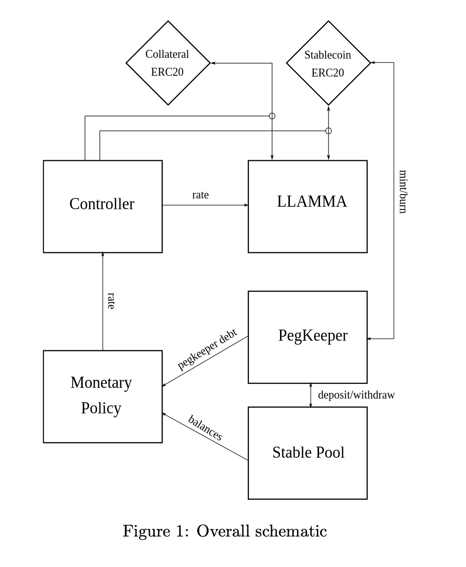
The entire protocol is composed of the following components (the following image is excerpted from the whitepaper):

• LLAMMA (Lending-Liquidating AMM Algorithm) is a specially designed AMM for liquidation. The name is a play on words for 'llama' (the mascot of the Curve community).

• Controller is responsible for user interaction logic and managing user liquidity in LLAMMA.

• Monetary Policy is a contract used to dynamically adjust the interest rate of the stablecoin.

• PegKeeper is a set of contracts designed to help stabilize the price of crvUSD.

• Stable Pool is the pool for crvUSD in Curve V1.

• Arbitrageurs help in the liquidation of user assets by arbitraging against LLAMMA.

LLAMMA

Among the many components of Curve Stablecoin, the most core component is LLAMMA, which is an AMM specifically designed for liquidation.

Suppose crvUSD uses ETH as collateral; then, LLAMMA would be a crvUSD-ETH AMM.

LLAMMA utilizes a design similar to Uniswap V3. For example, like Uniswap V3, LLAMMA uses ranges (called bands in LLAMMA) to segment liquidity, allowing users to provide liquidity to a specific range within the AMM.

However, a significant difference between LLAMMA and Uniswap V3 is the pattern of how the balances of the two tokens in the AMM pool change with price, as exemplified by ETH/USD:

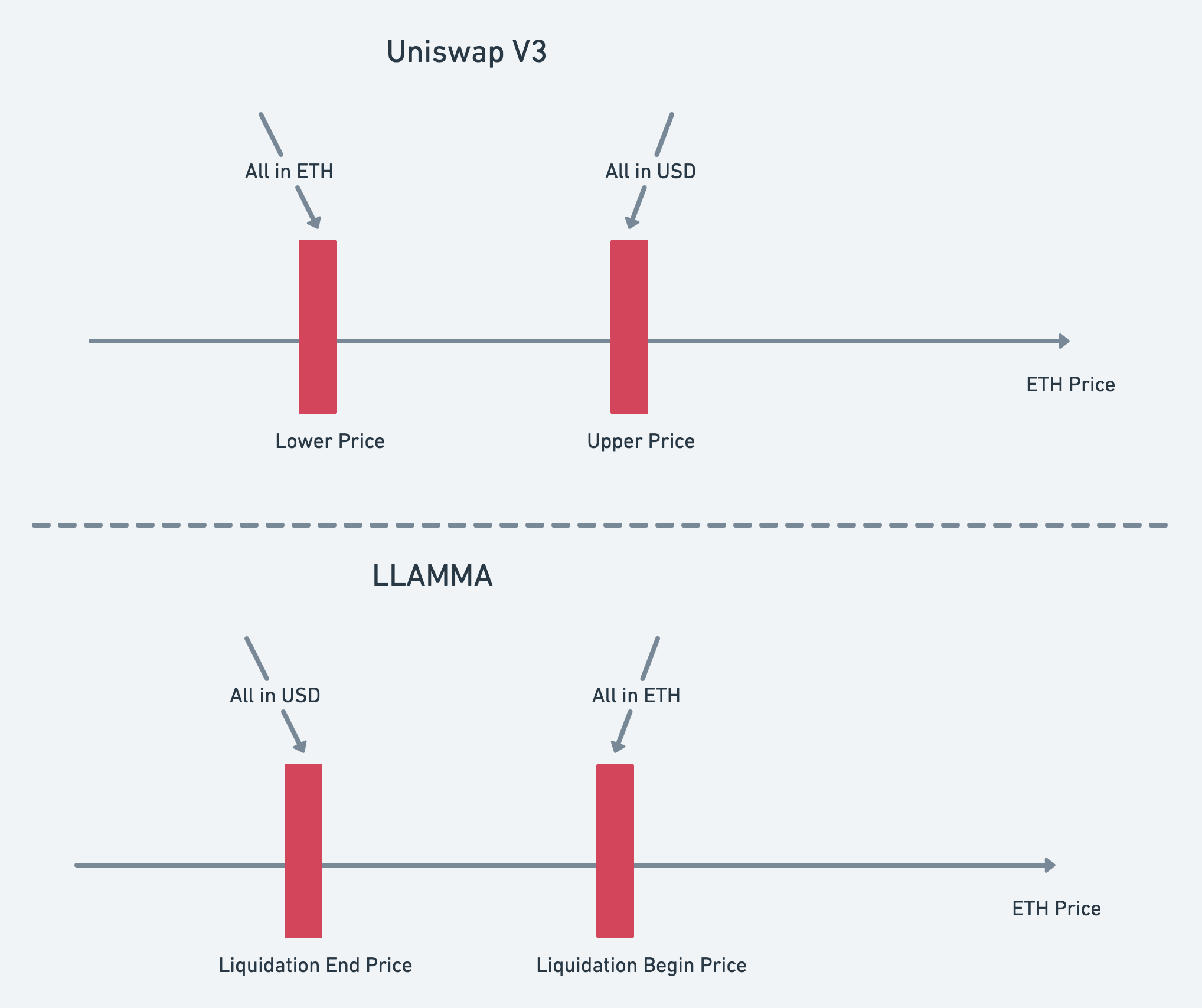
In Uniswap V3 (as depicted in the upper half of the dashed line in the diagram), users choose to provide liquidity within a range from Lower to Upper Price. This range is referred to as a range in Uniswap. When the ETH price is greater than or equal to the Upper Price, all of the user's liquidity will be in USD. As the price falls, the USD in the user's liquidity is converted into ETH. When the ETH price is less than or equal to the Lower Price, all of the user's liquidity will be in ETH.

In LLAMMA (as shown in the lower half of the dashed line in the diagram), users collateralize ETH to borrow crvUSD. Their ETH is then added to a specific range (band) in LLAMMA to provide liquidity, where the upper and lower bounds of this band are the start/end prices of liquidation. Initially, the price will be above the Liquidation begin price of the band, and all liquidity in the band will be in ETH. As the price falls, ETH in the band starts to be converted into crvUSD. When the price falls to the lower bound price (external price) of the band, all of the user's assets will be converted into crvUSD.

It can be observed that in LLAMMA, the change in the token balance within a band is exactly the opposite of Uniswap. This achieves the purpose of liquidating user assets: when the price is high, the user's ETH assets remain untouched within the liquidity. As the price falls to the upper limit of the user's liquidity range, ETH begins to be converted into crvUSD. When the price falls to the lower limit of the range, all of the user's ETH is converted into crvUSD. Assuming the conversion yields more crvUSD than the user's debt, the protocol will not face bad debt risk, and the entire process does not require the involvement of liquidators from traditional lending protocols.

The advantages of this approach are:

• The AMM itself provides liquidity, reducing reliance on external liquidity (though not completely independent).

• Traditional lending protocol liquidators are not needed (but forced liquidation may still occur in extreme situations). The entire liquidation process is carried out with the rebalance of the AMM's internal balance as prices fall.

• Liquidation is continuous, not phased. Thus, each time a user's assets are sold, they are sold at a level closer to the external market price, minimizing the loss for the user.

• If prices rebound, crvUSD will be converted back into ETH, and the user's assets will be repurchased. This avoids permanent losses for the user in a volatile market (although even if prices return to their original levels, it's difficult to achieve completely lossless transactions, as LLAMMA always sells assets in the Pool at a discount).

LLAMMA Design

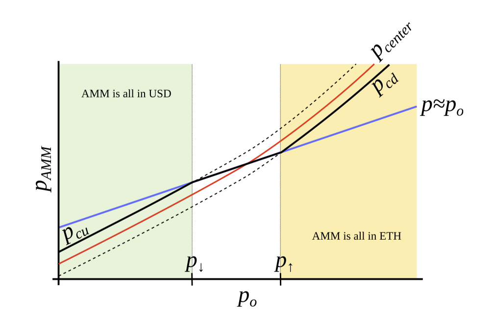
In the diagram, the horizontal axis $p_{o}p\_o$ represents the external price of ETH, while the vertical axis represents the internal price within the AMM. The blue line is a straight line with a slope of 1, indicating that the internal AMM price follows the changes in the external price. $p_{cu}p\_\{cu\}$ and $p_{cd}p\_\{cd\}$ represent the upper and lower bound prices of a particular band within the AMM, while $p_{\uparrow }p\_\uparrow$ and $p_{\downarrow }p\_\downarrow$ respectively represent two selected reference boundary prices in the external price coordinates.

We can find that when the external price $p_{o}p\_o$ increases, both $p_{cu}p\_\{cu\}$ and $p_{cd}p\_\{cd\}$ as well as the internal AMM price, will increase at a faster rate (forming a convex curve). Conversely, when the external price $p_{o}p\_o$ decreases, $p_{cu}p\_\{cu\}$ and $p_{cd}p\_\{cd\}$ along with the internal AMM price, will decrease at a faster rate.

Furthermore, when $p_o=p_{\uparrow }p\_o=p\_\uparrow$, $p_{cd}p\_\{cd\}$ precisely satisfies $p_{cd}=p_o=p_{\uparrow }p\_\{cd\}=p\_\{o\}=p\_\uparrow$, and when $p_o=p_{\downarrow }p\_o=p\_\downarrow$，$p_{cu}p\_\{cu\}$ precisely satisfies $p_{cu}=p_o=p_{\downarrow }p\_\{cu\}=p\_o=p\_\downarrow$.

If we can design an AMM that dynamically changes its range's upper and lower bound prices with the external price, then in this AMM:

• When the external price $p_o>=p_{\uparrow }p\_o\; >=\; p\_\uparrow$, the lower bound price of the band $p_{cd}>=p_{o}p\_\{cd\}\; >=\; p\_o$. This corresponds to the scenario in Uniswap V3 where the range is out of the money, and the external price is less than the range's lower bound. Just like in Uniswap V3, this range will be entirely ETH.
• When the external price , the upper bound price of the band . This corresponds to the scenario in Uniswap V3 where the range is out of the money, and the external price is higher than the range's upper bound. Thus, just like in Uniswap V3, this range will be entirely crvUSD.

This way, the AMM's range can have an internal balance change that is exactly the opposite of Uniswap V3 when $p_{o}p\_o$ fluctuates within the range of $[p_{\uparrow }-p_{\downarrow }][p\_\uparrow \; -\; p\_\downarrow ]$. Assuming the initial state is $p_o>p_{\uparrow }p\_o\; >\; p\_\uparrow$, as $p_{o}p\_o$ decreases to $p_{\uparrow }p\_\uparrow$, the ETH held by the user in the band begins to be converted into crvUSD, until $p_o=p_{\downarrow }p\_o\; =\; p\_\downarrow$, at which point all of the user's assets will have been converted into crvUSD.

LLAMMA Implementation

As previously mentioned, LLAMMA needs to know the external asset price $p_{o}p\_o$. In its actual implementation, LLAMMA uses the Oracle price from Curve V2 and applies EMA (exponential moving average) processing to it. LLAMMA predefines a continuous series of prices on the external price coordinate, which forms a geometric sequence. Users can select any two prices as the upper and lower reference prices for their liquidity ($p_{\downarrow }p\_\downarrow$ and $p_{\uparrow }p\_\uparrow$) Therefore, we have:

$\frac{p_{\downarrow }}{p_{\uparrow }}=\frac{A-1}{A}\backslash frac\{p\_\downarrow \}\{p\_\uparrow \}\; =\; \backslash frac\{A-1\}\{A\}$

Where $AA$ is a constant greater than 1, set when the LLAMMA pool is created. The larger the value of $AA$, the smaller the ratio between the boundary prices on the external price coordinate, resulting in a denser distribution. Currently, the value of $AA$ most of the markets is 100. This design is similar to the tick design in Uniswap, but it is important to note that here, $p_{\downarrow }p\_\downarrow$ and $p_{\uparrow }p\_\uparrow$ refer to the external prices, not the internal AMM prices. In its specific design, LLAMMA also satisfies an equation similar to Uniswap V3:

$I=(x+f)(y+g)I\; =\; (x\; +\; f)(y\; +\; g)$

Where $xx$ represents crvUSD and $yy$ represents ETH. As with Uniswap V3, the price in the AMM (ETH price) can be represented as:

$p=\frac{x+f}{y+g}p\; =\; \backslash frac\{x\; +\; f\}\{y\; +\; g\}$

Unlike Uniswap, in the equation above, both $ff$ and $gg$ are dynamic variables and are related to the external price $p_{o}p\_o$ ​. The functions for $ff$ and $gg$ are as follows:

$f=\frac{p_o^2}{p_{\uparrow }}A{y}_{0}g=\frac{p_{\uparrow }}{p_o}(A-1)y_{0}f\; =\; \backslash frac\{p\_o^2\}\{p\_\uparrow \}Ay\_0\backslash \; \backslash \; g=\backslash frac\{p\_\uparrow \}\{p\_o\}(A-1)y\_0$

In the formulas, $y_{0}y\_0$ represents the amount of ETH in the interval when $p_o=p_{\downarrow }p\_o\; =\; p\_\downarrow$. In this state, the AMM's token balance satisfies: $y=y_{0}y\; =\; y\_0$, $x=0x\; =\; 0$. Here we can initially assume $y_{0}y\_0$ is a constant (actually, $y_{0}y\_0$ is not a constant, but we can ignore its change for now), and in the formula, $p_{\uparrow }p\_\uparrow$ and $AA$ are also constants. Michael did not provide the design process for these two functions, but we can see the purpose of such a design:

As the external price $p_{o}p\_o$ increases, $ff$ grows exponentially and $gg$ decreases. Conversely, when $p_{o}p\_o$ decreases, $ff$ decreases exponentially, and $gg$ increases.

Combining this with the AMM price formula $p=\frac{f+x}{g+y}p\; =\; \backslash frac\{f+x\}\{g+y\}$, we can see that as the external price $p_{o}p\_o$ rises, the internal price $pp$ within LLAMMA also rises, and the rate of increase is much higher than that of the external price increase (the denominator decreases while the numerator increases exponentially). Conversely, when the external price $p_{o}p\_o$ falls, the internal price $pp$ within LLAMMA drops more rapidly.

Thus, LLAMMA achieves its first characteristic: even without any trades, the internal price in LLAMMA automatically changes with the external price, and it changes at a faster rate.

Through this method of automatically adjusting the AMM price, the token balance within LLAMMA exhibits the opposite behavior of Uniswap V3 in response to price changes. For example, when the external price of ETH falls:

• In Uniswap, the internal price remains unchanged, and arbitrageurs will sell ETH in Uniswap at a relatively higher price, therefore the amount of ETH in the Uniswap Pool increases while USD decreases.

• In LLAMMA, the internal price will fall more than the external price, arbitrageurs will buy ETH in LLAMMA at a relatively lower price, therefore the amount of ETH in the LLAMMA Pool decreases while USD increases.

It can be seen that when the price falls, LLAMMA attracts arbitrageurs by creating a price difference. The act of arbitrageurs buying ETH from LLAMMA is essentially liquidating the user's assets, and the profit of the arbitrageurs is the buying price difference.

Similarly, when the price falls to the liquidation range and then begins to rebound, LLAMMA also raises the internal price through the price difference, allowing arbitrageurs to sell ETH back into the LLAMMA pool, and helping users repurchase their assets.

However, LLAMMA may not necessarily help users buy back all of their original collateralized assets. This is due to the AMM Path Dependence problem caused by LLAMMA's proactive change in AMM price (which can be referred to in this Tweet). Simply put, as the external price moves, LLAMMA is continuously giving profits to arbitrageurs (selling low and buying high), which will cause the loss of user assets, even if prices return, the LLAMMA state is difficult to restore.

It is also worth noting that due to the exponential relationship between LLAMMA's internal price changes and external prices, if the intervention by arbitrageurs is not timely enough, or the external price changes are too large, it will cause a significant price difference between LLAMMA and the external market, increasing the user's losses. To avoid large fluctuations in the external price, Curve uses an EMA to process the external Oracle price before providing it to LLAMMA. To learn more about Curve oracle features see the Oracle section.

Swap Calculation

When $p_o=p_{\uparrow }p\_o\; =\; p\_\uparrow$, the entire band consists of ETH, and the amount of ETH is $y_{0}y\_0$, the token balance state within the AMM is $y=y_{0}y\; =\; y\_0$, $x=0x\; =\; 0$. Substituting $ff$ and $gg$ into the identity, we get:

$I=p_o{A}^2{y}_0^{2}I\; =\; p\_o\; A^2\; y\_0^2$

Extending this identity to any price $p_{o}p\_o$ within the range of $p_{\uparrow }\sim p_{\downarrow }p\_\uparrow \; \backslash sim\; p\_\downarrow$

$(\frac{p_o^2}{p_{\uparrow }}A{y}_0+x)(\frac{p_{\uparrow }}{p_o}(A-1)y_0+y)=p_o{A}^2{y}_0^2\backslash left(\backslash frac\{p\_o^2\}\{p\_\uparrow \}\; A\; y\_0\; +\; x\backslash right)\backslash left(\backslash frac\{p\_\uparrow \}\{p\_o\}\; (A\; -\; 1)y\_0\; +\; y\backslash right)\; =\; p\_o\; A^2\; y\_0^2$

As previously mentioned, $y_{0}y\_0$ is not a constant; in fact, it is also a function of $p_{o}p\_o$.

The above formula can be written as a quadratic equation in terms of $y_{0}y\_0$:

$p_{o}A{y}_0^2-y_0(\frac{p_{\uparrow }}{p_o}(A-1)x+\frac{p_o^2}{p_{\uparrow }^2}Ay)-xy=0p\_o\; A\; y\_0^2\; -\; y\_0\; \backslash left(\backslash frac\{p\_\uparrow \}\{p\_o\}\; (A\; -\; 1)x\; +\; \backslash frac\{p\_o^2\}\{p\_\uparrow ^2\}\; Ay\backslash right)\; -\; xy\; =\; 0$

At any moment, we know the balances of $x,yx,\; y$ in the AMM, the external price $p_{o}p\_o$ and the reference upper limit price $p_{\uparrow }p\_\uparrow$ of the band, then we can solve for the unknown $y_{0}y\_0$ in this equation.

In the Curve contract, the code for solving $y_{0}y\_0$ corresponds to the AMM.get_y0() function:

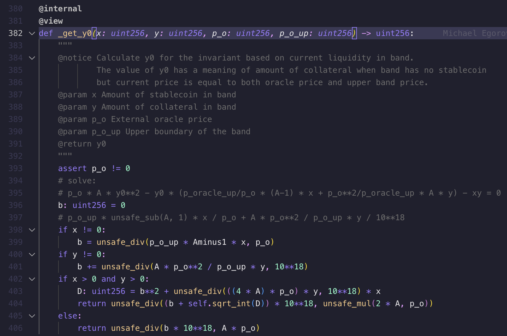
After calculating $y_{0}y\_0$, the aforementioned formula can be used to calculate the output amount for a trader swapping in the AMM. In the Curve contract, the code for calculating the swap output amount corresponds to the AMM.calc_swap_out() function. This is a very lengthy function, so for brevity, the specific code implementation is not shown here.

A simple description of the calculation process for an $x\to yx\; \backslash rightarrow\; y$ swap:

1. Find the band closest to the current price that has liquidity.
2. Read the values of $xx$ and $yy$ within the band, and calculate $y_{0}y\_0$.
3. Calculate the needed $\mathrm{\Delta }x\backslash Delta\; x$ when $y=0y\; =\; 0$.
4. If $\mathrm{\Delta }x\backslash Delta\; x$ is less than or equal to the $x_{in}x\_\{in\}$ - swap input amount, then the user swaps in this band and gets $yy$. Then, start from step 1 and enter the next band for another swap.
5. If $\mathrm{\Delta }x\backslash Delta\; x$ is greater than $x_{in}x\_\{in\}$, the swap input amount, then set $x=x+x_{in}x\; =\; x\; +\; x\_\{in\}$, calculate $\mathrm{\Delta }y\backslash Delta\; y$, and end the swap.

The amount of $yy$ obtained by the user is the sum of the results calculated in all the bands passed through during this swap. If the swap is $y\to xy\; \backslash rightarrow\; x$, the calculation process is largely the same.

Note that in this process, the swap calculations within a band treat $y_{0}y\_0$ as a fixed value (using the state before the swap). This makes the engineering implementation easier and the error will not be too large, provided the distance between bands is not too wide.

Band range price

For a given band, $p_{cu}p\_\{cu\}$ and $p_{cd}p\_\{cd\}$ are the upper and lower limit prices of the band within the AMM, respectively. When the internal AMM price reaches the upper limit price $p_{cu}p\_\{cu\}$, similar to Uniswap V3, the internal $y=0y\; =\; 0$ within the band. When the AMM price reaches the lower limit price $p_{cd}p\_\{cd\}$, the internal $x=0x\; =\; 0$ within the band. By substituting $x=0x\; =\; 0$ into LLAMMA's invariant, we can solve for $yy$, and at this point, the AMM's price is the lower limit price $p_{cd}p\_\{cd\}$. Similarly, the AMM price at $y=0y\; =\; 0$ represents the band's upper limit price $p_{cu}p\_\{cu\}$. Simplifying these two price formulas, we get:

$p_{cd}=\frac{p_o^3}{p_{\uparrow }^2},p_{cu}=\frac{p_o^3}{p_{\downarrow }^2}p\_\{cd\}\; =\; \backslash frac\{p\_o^3\}\{p\_\uparrow ^2\},\; \backslash quad\; p\_\{cu\}\; =\; \backslash frac\{p\_o^3\}\{p\_\downarrow ^2\}$

For a band, $p_{\downarrow }p\_\downarrow$ and $p_{\uparrow }p\_\uparrow$ are fixed values, so the $p_{cd}p\_\{cd\}$ and $p_{cu}p\_\{cu\}$ within the band depend only on the external price $p_{o}p\_o$.

We can identify the second characteristic of LLAMMA: the upper and lower limit prices of a band within LLAMMA also automatically change with the external price, and the rate of change is faster. Let's illustrate these two characteristics of LLAMMA with a diagram (image captured from desmos):

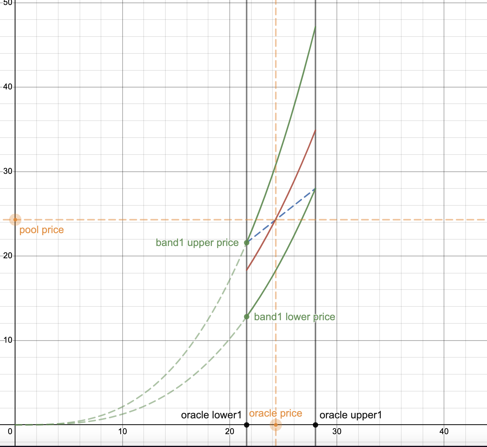
In the diagram, the horizontal axis represents the external price, and the vertical axis represents the internal price of the AMM. The black solid line represents the reference external upper limit price for a band ($p_{\downarrow }p\_\downarrow$ and $p_{\uparrow }p\_\uparrow$), the green solid line represents the upper and lower limit prices of this band ($p_{cu}p\_\{cu\}$ and $p_{cd}p\_\{cd\}$), the blue dashed line is a dashed line with a slope of 1, indicating that the AMM price $pp$ is equal to the external price $p_{o}p\_o$, and the red solid line represents the internal price of the AMM.

We can observe that as the external price increases, both the upper and lower limit prices of the band and the internal price of the AMM increase at a faster rate, and the internal price of the AMM is always within the upper and lower limit prices of the band.

Relationship Between Bands

When creating an LLAMMA pool, a starting reference price, $p_{\text{base}}p\_\{\backslash text\{base\}\}$, needs to be set. Subsequently, all $p_{\uparrow }p\_\uparrow$ and $p_{\downarrow }p\_\downarrow$ can be calculated, depending on the band number - $nn$:

$p_{\uparrow }(n)={\left(\frac{A-1}{A}\right)}^n{p}_{\text{base}},p_{\downarrow }(n)={\left(\frac{A-1}{A}\right)}^{n+1}{p}_{\text{base}}p\_\uparrow (n)\; =\; \backslash left(\backslash frac\{A-1\}\{A\}\backslash right)^n\; p\_\{\backslash text\{base\}\},\; \backslash quad\; p\_\downarrow (n)\; =\; \backslash left(\backslash frac\{A-1\}\{A\}\backslash right)^\{n+1\}\; p\_\{\backslash text\{base\}\}$

Since $p_{\uparrow }p\_\uparrow$ and $p_{\downarrow }p\_\downarrow$ are fixed values, once the value of $p_{o}p\_o$ is determined, the upper and lower limit prices $p_{cu}p\_\{cu\}$ and $p_{cd}p\_\{cd\}$ in each band can be known.

This diagram shows the relationship between three bands (image captured from desmos):

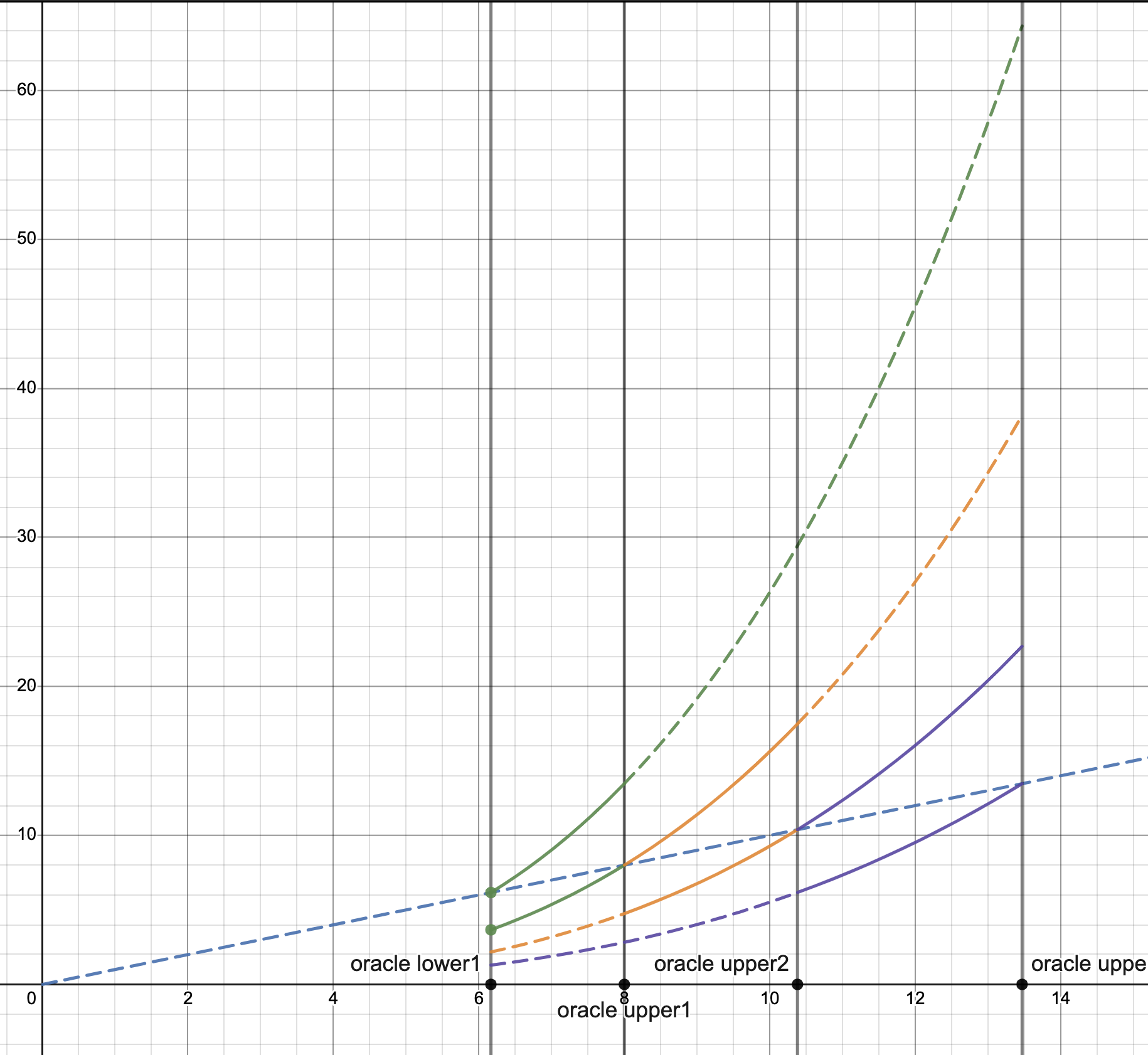
In the diagram, the horizontal axis represents the external price, while the vertical axis represents the internal price. The blue dashed line is a straight line with a slope of 1. The diagram includes four predefined reference external upper limit prices, which form three bands. In each band, the upper and lower limit prices within the AMM are represented by green, orange, and purple curves, respectively. The solid lines indicate that the band is expected to be in an active state, meaning it can be used for swaps (liquidation), while the dashed lines suggest that the band is likely to be out of the money, either not yet started for swaps or already completely swapped.

Upon closer examination, you can see that the blue dashed line intersects each band at the points where $p_{cu}=p_{\downarrow }p\_\{cu\}\; =\; p\_\downarrow$ and $p_{cd}=p_{\uparrow }p\_\{cd\}\; =\; p\_\uparrow$. This ensures that internal price will always be within the respected price range (between $p_{cd}p\_\{cd\}$ and $p_{cu}p\_\{cu\}$ curves).

Moreover, $p_{cd}p\_\{cd\}$ of the previous band will coincide with $p_{cu}p\_\{cu\}$ of the next band, ensuring that there are no gaps between the bands and that the liquidity within the bands is continuous across the internal price range of the AMM.

The following formulas can represent the aforementioned relationship:

$p(x=0,y>0,n)=p_{cd}(n)=p_{cu}(n-1)p(x\; =\; 0,\; y\; >\; 0,\; n)\; =\; p\_\{cd\}(n)\; =\; p\_\{cu\}(n\; -\; 1)$
$p(x>0,y=0,n)=p_{cu}(n)=p_{cd}(n+1)p(x\; >\; 0,\; y\; =\; 0,\; n)\; =\; p\_\{cu\}(n)\; =\; p\_\{cd\}(n\; +\; 1)$

In the diagram, it can also be observed that in the external price range, the $p_{cu}p\_\{cu\}$ and $p_{cd}p\_\{cd\}$ in the bands with lower external prices (on the left) are actually higher than the $p_{cu}p\_\{cu\}$ and $p_{cd}p\_\{cd\}$ in the bands at higher external prices (on the right).

Liquidation/Redemption Outcome Estimation

In actual contracts, users' funds will be deposited into a group of continuous bands (at least 4). The $p_{\uparrow }p\_\uparrow$ of largest band then becomes the start price for the liquidation of the user's assets, and $p_{\downarrow }p\_\downarrow$ of the smallest band is the end price for the liquidation. When this price is reached, all of the user's ETH will be converted into crvUSD. When users deposit ETH to mint crvUSD, Curve needs to help users choose a suitable group of bands to deposit their ETH into. These bands should meet the requirement: when all the user's ETH is converted into crvUSD, the amount of crvUSD obtained should be greater than the user's debt (in actual contracts, a coefficient is multiplied to leave some margin). This is to ensure that the protocol does not incur a bad debt.

Therefore, an estimation needs to be made when users deposit ETH into the bands: the amount of crvUSD obtained after all the ETH in the bands is traded into crvUSD as the external price of ETH decreases, which we denote as $x_{\downarrow }x\_\downarrow$. Similarly, we can estimate the amount of ETH obtained when the external price rebounds and all the crvUSD in the bands is traded back into ETH, denoted as $y_{\uparrow }y\_\uparrow$.

The estimation formula provided by Curve:

$y_{\uparrow }=y+\frac{x}{\sqrt{p_{\uparrow }p}}y\_\uparrow \; =\; y\; +\; \backslash frac\{x\}\{\backslash sqrt\{p\_\uparrow \; p\}\}$

$x_{\downarrow }=x+y\sqrt{p_{\downarrow }p}x\_\downarrow \; =\; x\; +\; y\; \backslash sqrt\{p\_\downarrow \; p\}$

This set of formulas uses the most optimistic estimation method, that is, estimating the maximum possible outcome. Previously, we mentioned that changes in external prices lead to changes in LLAMMA prices, creating a price difference with external prices. The entry of arbitrageurs causes losses to users. To estimate the maximum value of the results, we need to assume:

• The external price changes at an extremely slow pace, meaning that over a certain period, the price difference between the external price and the internal price in LLAMMA is minimal and can be ignored.

• Traders conduct transactions in LLAMMA, causing the internal price of LLAMMA to change synchronously with the external price. Since the price difference between the AMM internal price and the external price can be ignored, users will not incur losses due to price differences during the trading process.

These two assumptions correspond to the meaning of 'adiabatically' as described in the Curve whitepaper. 'Adiabatically' in physics denotes a process occurring without heat transfer. In this context, we can understand it as an ideal state that isolates arbitrage transactions due to price differences.

In such an ideal state, LLAMMA can directly use the Uniswap V3 formulas to calculate the swap results, which are the aforementioned two formulas. The derivation process for these formulas is:

$$y_{\uparrow }=y+\mathrm{\Delta }yy\_\backslash uparrow\; =\; y\; +\; \backslash Delta\; y$$ $$=y+\sqrt{I}(\frac{1}{\sqrt{p_{\uparrow }}}-\frac{1}{\sqrt{p}})=\; y\; +\; \backslash sqrt\{I\}\; \backslash left(\backslash frac\{1\}\{\backslash sqrt\{p\_\backslash uparrow\}\}\; -\; \backslash frac\{1\}\{\backslash sqrt\{p\}\}\backslash right)$$ $$=y+\frac{\sqrt{Ip}-\sqrt{I{p}_{\uparrow }}}{p_{\uparrow }p}=\; y\; +\; \backslash frac\{\backslash sqrt\{I\; p\}\; -\; \backslash sqrt\{I\; p\_\backslash uparrow\}\}\{p\_\backslash uparrow\; p\}$$ $$=y+\frac{(f+x)-f}{\sqrt{p_{\uparrow }p}}=\; y\; +\; \backslash frac\{(f\; +\; x)\; -\; f\}\{\backslash sqrt\{p\_\backslash uparrow\; p\}\}$$ $$=y+\frac{x}{\sqrt{p_{\uparrow }p}}=\; y\; +\; \backslash frac\{x\}\{\backslash sqrt\{p\_\backslash uparrow\; p\}\}$$ $$x_{\downarrow }=x+\sqrt{I}(\sqrt{p_{\downarrow }}-\sqrt{p})x\_\backslash downarrow\; =\; x\; +\; \backslash sqrt\{I\}\; \backslash left(\backslash sqrt\{p\_\backslash downarrow\}\; -\; \backslash sqrt\{p\}\backslash right)$$ $$=x+\sqrt{I}(\frac{1}{\sqrt{p}}-\frac{1}{\sqrt{p_{\downarrow }}})\sqrt{p_{\downarrow }p}=\; x\; +\; \backslash sqrt\{I\}\; \backslash left(\backslash frac\{1\}\{\backslash sqrt\{p\}\}\; -\; \backslash frac\{1\}\{\backslash sqrt\{p\_\backslash downarrow\}\}\backslash right)\; \backslash sqrt\{p\_\backslash downarrow\; p\}$$ $$=x+((g+y)-g)\sqrt{p_{\downarrow }p}=\; x\; +\; ((g\; +\; y)\; -\; g)\backslash sqrt\{p\_\backslash downarrow\; p\}$$ $$=x+y\sqrt{p_{\downarrow }p}=\; x\; +\; y\; \backslash sqrt\{p\_\backslash downarrow\; p\}$$

Through this estimation method, the Controller contract will help users add liquidity to the appropriate band based on the user's debt, collateral value, and the selected band width.

Furthermore, with the estimation of liquidation/redemption outcomes, it is possible to know at any given moment whether the user's assets, after being completely swapped, will be sufficient to repay the debt. If at any point it is found that the user's assets, even if entirely swapped into crvUSD, are not enough to cover the debt, liquidators need to intervene for a forced liquidation. The specific process is similar to the traditional lending liquidation process, which is not elaborated further in this text.

When $p=p_{\uparrow }=p_{cd}p\; =\; p\_\uparrow \; =\; p\_\{cd\}$, $x=0x\; =\; 0$ within the AMM. Therefore, $x_{\downarrow }=y\sqrt{p_{\downarrow }{p}_{\uparrow }}x\_\downarrow \; =\; y\; \backslash sqrt\{p\_\downarrow \; p\_\uparrow \}$, this means that ideally, within a band, the average selling price of user assets is the geometric mean of the reference upper and lower limit prices of this band: $\sqrt{p_{\downarrow }{p}_{\uparrow }}\backslash sqrt\{p\_\downarrow \; p\_\uparrow \}$. Similarly, the price at which user assets are redeemed is also this geometric mean.

The functions in the contract related to the above description include Controller.get_y_effective(), AMM.get_x_down(), AMM.get_y_up(), Controller.liquidate(), etc. Due to space limitations, the details of the code implementation are not explained here.

LLAMMA Summary

We summarize the characteristics of LLAMMA:

• The LLAMMA Pool contains predefined continuous bands. When adding liquidity, tokens can be added to a group of bands.
• Bands are determined by the external reference prices $p_{\uparrow }p\_\uparrow$ and $p_{\downarrow }p\_\downarrow$, which form a geometric sequence between them.
• Within the AMM, $p_{cu}p\_\{cu\}$ and $p_{cd}p\_\{cd\}$ represent the upper and lower limit prices of a band in the AMM.
• The LLAMMA AMM price, along with all the $p_{cu}p\_\{cu\}$ and $p_{cd}p\_\{cd\}$ of the bands, increases as the external price $p_{o}p\_o$ increases, and the rate of change is faster. The same is true in reverse.
• When users create debt, their assets are stored in a group of bands (these bands are always outside the AMM price, so only ETH is added).
• When the ETH price falls, reaching the upper reference price $p_{\uparrow }p\_\uparrow$ of the largest band in user liquidity, theoretically (assuming enough arbitrageurs and traders), $p=p_{cd}=p_{\uparrow }p\; =\; p\_\{cd\}\; =\; p\_\uparrow$ is satisfied, and the user's assets begin to be liquidated.
• If the ETH price continues to fall, reaching the lower reference price $p_{\downarrow }p\_\downarrow$ of the smallest band in user liquidity, theoretically $p=p_{cu}=p_{\downarrow }p\; =\; p\_\{cu\}\; =\; p\_\downarrow$ is satisfied, and all the user's assets are liquidated into crvUSD.
• If the ETH price begins to rebound, LLAMMA will help users buy back their collateralized assets, ETH.
• LLAMMA only exposes the swap interface to the outside and does not directly expose interfaces for adding/removing liquidity to users. Therefore, users cannot arbitrarily add liquidity to LLAMMA without creating debt, and these related operations are managed by a dedicated Controller.

Controller

The Controller implements user interaction interfaces externally, while internally it interfaces with LLAMMA, responsible for depositing/withdrawing user assets into/from LLAMMA.

When users create debt by depositing, they need to specify these parameters:

• The amount of ETH collateral.

• The size of the crvUSD debt being created.

• The number of continuous bands in LLAMMA into which the ETH is deposited.

The third parameter, the number of bands, must be at least 4 and at most 50. The Controller calculates the bands in which the user needs to deposit based on these three parameters and deposits the user's ETH into these bands (these bands are always out of the money, so liquidity is added as ETH only). Simultaneously, crvUSD is sent to the user, and the user's debt is equal to the amount of crvUSD minted.

This process utilizes the liquidation outcome estimation formulas mentioned earlier. In the contract, the corresponding function is Controller.create_loan().

In addition, the Controller also has functions for adding collateral, repaying debt, withdrawing collateral, forced liquidation, maintaining loan interest, etc. These functions are not elaborated upon in this text.

PegKeeper

PegKeeper, also known as the stabilizer, is a set of contracts designed to help maintain the peg of crvUSD's price. These contracts primarily interact with the Curve V1 pool.

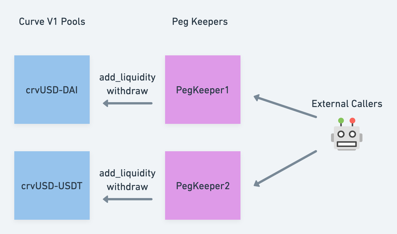
After the launch of crvUSD, corresponding pools will be created in Curve V1. For simplicity in this example, let's assume crvUSD creates individual Curve V1 pools with DAI and USDT. Suppose the price of crvUSD is $p_{s}p\_s$:

• When $p_s>1p\_s\; >\; 1$ it indicates a shortage of crvUSD supply. PegKeeper will mint crvUSD and add it to the Curve V1 pool (adding crvUSD as a single asset), to increase the market supply of crvUSD.
• When it indicates an excess supply of crvUSD. PegKeeper will remove the previously added liquidity from the Curve V1 pool (removing crvUSD as a single asset), to reduce the market supply of crvUSD.

The process is illustrated in the following diagram:

PegKeeper, in the process of carrying out these operations, functions similarly to 'buy low, sell high,' and can generate profits. For example:

When $p_s>1p\_s\; >\; 1$ it indicates that there is a shortage of crvUSD in the Curve V1 pool. External accounts can call the PegKeeper contract to mint crvUSD and add it to the Curve V1 pool (adding crvUSD as a single asset). It's important to note that the minted crvUSD, being uncollateralized and created out of thin air, can only be added to the Curve V1 pool by PegKeeper. The total amount minted is recorded as a debt of the PegKeeper contract.

After the price $p_{s}p\_s$ stabilizes or when $p_s>1p\_s\; >\; 1$ external accounts can call the PegKeeper contract to withdraw the previously added liquidity from the Curve V1 pool. The withdrawal only removes crvUSD as a single asset and repays the debt previously incurred by PegKeeper.

PegKeeper's actions of adding/removing crvUSD in Curve V1 are all done as single asset transactions, directly influencing the price of crvUSD in the Curve V1 pool to bring it closer to the pegged price.

Additionally, since crvUSD is added when its price is high and removed when it is low, PegKeeper will have surplus LP tokens after repaying its debts. These LP tokens represent the profits generated by PegKeeper. A portion of these profits is distributed to external callers as gas compensation and incentives each time they call the PegKeeper contract. The remaining profits are retained as protocol revenue.

However, external callers can not arbitrarily call PegKeeper. The contract has a series of checks to prevent malicious calls and ensure that the calls enable PegKeeper to generate profits.

It is important to note that PegKeeper's capacity to respond to market conditions is not entirely symmetrical in dealing with both scenarios:

• When $p_s>1p\_s\; >\; 1$ PegKeeper can mint crvUSD out of thin air without collateral and add it to the Curve V1 pool for market regulation. Since PegKeeper doesn't require collateral, its market regulation capacity is theoretically unlimited in this scenario.
• When PegKeeper can only remove the liquidity previously added to the Curve V1 pool for market regulation. At this time, PegKeeper's capacity is limited by the amount of crvUSD minted when $p_s>1p\_s\; >\; 1$. If PegKeeper had not minted any crvUSD previously, or if the price of crvUSD is still less than 1 after removing all liquidity, it leads to a situation as in Chinese proverb: even the cleverest housewife can't cook rice without rice.

Therefore, to compensate for the insufficiency of PegKeeper's capacity when Curve Stablecoin also needs to adjust interest rates as a further means to help peg the price of crvUSD.

Monetary Policy

A dynamic component for adjusting lending rates, used to regulate interest rates based on market supply and demand, further helping to stabilize the price anchoring of crvUSD, primarily used in scenarios where the crvUSD price .

The logic for interest rates implemented in the open-source code of Curve Stablecoin is slightly different from that described in the whitepaper. Here, I will explain it according to the logic in the actual code.

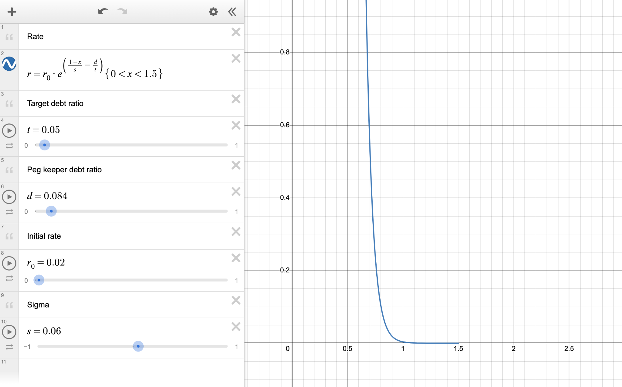
We denote the total debt generated by PegKeeper as $d_{pk}d\_\{pk\}$, and the total debt generated by users through the Controller as $d_{t}d\_t$, The ratio of these two debts is denoted as $r_{d}r\_d$. The price of crvUSD is denoted $pp$, and we define a base interest rate $r_{0}r\_0$. The interest rate for crvUSD is:

$r=r_0\cdot e^{(\frac{1-p}{\sigma }-\frac{r_d}{\alpha })}r\; =\; r\_0\; \backslash cdot\; e^\{\backslash left(\backslash frac\{1-p\}\{\backslash sigma\}\; -\; \backslash frac\{r\_d\}\{\backslash alpha\}\backslash right)\}$

In the above equation, $\sigma \backslash sigma$ is a constant, and $\alpha \backslash alpha$ is the target debt ratio.

After setting specific values for these parameters (currently, in Monetary Policy for ETH market $\sigma \backslash sigma$ is set to 0.02 and target debt ratio equals 0.1), the curve of the interest rate changes with the price is illustrated in the following diagram (screenshot from desmos):

We can observe:

• When the price of crvUSD is greater than 1, the interest rate is relatively low.

• When the price of crvUSD is less than 1, the interest rate sharply increases after a certain critical point (the rate of increase depends on $\sigma \backslash sigma$)

The reason for this design:

• If the price of crvUSD is greater than 1, PegKeeper has sufficient capacity to regulate the market. In this case, maintaining a low-interest rate helps attract more users to mint crvUSD.

• If the price of crvUSD is less than 1, PegKeeper’s capacity is limited. At this point, to reduce the market supply of crvUSD, it is necessary to raise the interest rate to force users to repay their debts. To avoid excessive price differences caused by detethering, the rate of interest increase will begin to rise rapidly after crvUSD falls below a certain critical point. The rate of increase depends on the $\sigma \backslash sigma$ parameter, and the price at which the interest rate starts to increase depends on the size of PegKeeper’s debt.

Additionally, we can observe the impact of the parameter and the PegKeeper debt ratio $r_{d}r\_d$ on the actual interest rate changes:

It can be seen that the closer $\sigma \backslash sigma$ is to 0, the steeper the curve becomes, and the faster the interest rate increases as the price decreases.

When the proportion of PegKeeper's debt is relatively large, it shifts the curve to the left, making the interest rate start to rise at a lower price.

The reason for this approach is that if PegKeeper's debt proportion is large, it indicates that PegKeeper holds a significant amount of liquidity in Curve V1. When the price of crvUSD is less than 1, PegKeeper can first remove liquidity (crvUSD as a single asset) from Curve V1 to reduce its debt, simultaneously aiding the price of crvUSD to return to its peg. The larger the debt of PegKeeper, the more the price of crvUSD needs to fall before the interest rate begins to rise rapidly. This approach helps PegKeeper control the size of its debt.

Oracle

As mentioned earlier, Curve Stablecoin in LLAMMA needs to know the external price of the collateral ETH, and in PegKeeper and Monetary Policy, it needs to know the external price of crvUSD. For the collateral price, Curve will fetch it from the Curve V2 pool, and the crvUSD price will be fetched from the corresponding Curve V1 pools (referring to prices in multiple pools).

Before using external prices, Curve Stablecoin first processes these prices with an Exponential Moving Average (EMA). As previously stated, if there are significant fluctuations in the external Oracle prices, then a substantial price difference between LLAMMA prices and external prices can occur, resulting in losses for users. Using EMA prices can help reduce price volatility and also increase the difficulty of manipulating Oracle prices.

Oracles functionality is updated based on changing market conditions and analysis of the influence of various parameters on the operation of the protocol. Thereby, the second version of oracles for crvUSD takes into account TVLs of aggregated pools and adjusts weights based on that.

Collateral oracles fetch prices from pools and to prevent manipulations through flash loans, Curve employed a hybrid approach using TriCrypto, Chainlink, and Uniswap Twap Oracle prices, instead of solely relying on TriCrypto prices. Oracle price is checked against anchor price (from Chainlink or Uni TWAP oracles). There is a threshold for price deviation, called safety limit, and if the price difference hits the threshold, then the oracle uses the price from the anchor source. However, the Curve team did research showing that Chainlink (or, rather, market spot) prices cause more losses than necessary in periods of high volatility. So, there was a proposal for disabling Chainlink limits.

FAQs

Below are some common questions about Curve Stablecoin:

How can liquidity be provided to LLAMMA?

Users can only add liquidity to LLAMMA through the Controller, by pledging ETH to create crvUSD debt. The ETH will be added to LLAMMA by the Controller. Ordinary users don't have to consider market making in LLAMMA, as the characteristics of LLAMMA mean that its Liquidity Providers (LPs) are very likely to incur losses in trading.

When minting crvUSD requires collateralizing ETH to provide liquidity to LLAMMA, where is the user's ETH placed?

Users need to specify the number of bands they wish to enter. Subsequently, the Controller, based on the user's debt size, automatically selects a group of bands that minimizes the user's risk. This group consists of the bands with the lowest prices, while also ensuring that the protocol does not face bad debt risk.

How is the number of bands chosen?

When creating debt, users need to decide the number of bands into which their ETH will be placed.

When minting the same amount of crvUSD, the greater the number of bands, the more dispersed the collateral distribution, leading to a higher starting price for liquidation. Conversely, fewer bands result in more concentrated collateral distribution, with a relatively lower starting price for liquidation.

If a higher loan-to-value ratio is desired, fewer bands should be chosen, but this also increases the risk of liquidation.

How does Curve specifically add a user's ETH to LLAMMA when they mint crvUSD?

• Since the user's collateral is only ETH, this definitely involves single-sided liquidity, meaning the band contains only ETH.

• Curve will try to add the user's ETH to bands with lower prices, but also needs to ensure that the protocol does not face bad debt risk.

Curve selects appropriate bands and adds liquidity based on the amount of ETH the user has, the width of the bands chosen by the user, and the amount of crvUSD minted. The specific logic is as follows:

Suppose the user's collateralized ETH amount is $yy$. We can use Formula 10 from the whitepaper to calculate the amount of crvUSD obtained when the user's ETH in a certain band is traded into crvUSD (for simplicity, we ignore loan_discount here):

$$x_{\downarrow }=y\sqrt{p_{\uparrow }{p}_{\downarrow }}=y{p}_{\uparrow }\sqrt{\frac{A-1}{A}}x\_\downarrow \; =\; y\; \backslash sqrt\{p\_\uparrow \; p\_\downarrow \}\; =\; yp\_\uparrow \; \backslash sqrt\{\backslash frac\{A-1\}\{A\}\}$$

In LLAMMA, the user's ETH is evenly distributed across $NN$ bands, with each band containing an amount of ETH equal to $\frac{y}{N}\backslash frac\{y\}\{N\}$. Assuming the band with the highest price is numbered $n1n1$, after using the above formula to calculate for each band and summing up the results, we can obtain:

$x_{\downarrow }=\frac{y{p}_{\uparrow }}{N}\cdot \sqrt{\frac{A-1}{A}}\cdot {\sum }_{k=0}^{N-1}{\left(\frac{A-1}{A}\right)}^{k}x\_\downarrow \; =\; \backslash frac\{yp\_\uparrow \}\{N\}\; \backslash cdot\; \backslash sqrt\{\backslash frac\{A-1\}\{A\}\}\; \backslash cdot\; \backslash sum\_\{k=0\}^\{N-1\}\; \backslash left(\backslash frac\{A-1\}\{A\}\backslash right)^k$

We define a variable $y_{\text{effective}}y\_\{\backslash text\{effective\}\}$ that is related only to the user's band width $NN$ and is independent of the band price:

$y_{\text{effective}}=\frac{y}{N}\cdot \sqrt{\frac{A-1}{A}}\cdot {\sum }_{k=0}^{N-1}{\left(\frac{A-1}{A}\right)}^{k}y\_\{\backslash text\{effective\}\}\; =\; \backslash frac\{y\}\{N\}\; \backslash cdot\; \backslash sqrt\{\backslash frac\{A-1\}\{A\}\}\; \backslash cdot\; \backslash sum\_\{k=0\}^\{N-1\}\; \backslash left(\backslash frac\{A-1\}\{A\}\backslash right)^k$

We also define $x_{\downarrow }x\_\downarrow$ as $x_{\text{effective}}x\_\{\backslash text\{effective\}\}$. The above formula simplifies to:

$x_{\text{effective}}=y_{\text{effective}}\cdot p_{\uparrow }x\_\{\backslash text\{effective\}\}\; =\; y\_\{\backslash text\{effective\}\}\; \backslash cdot\; p\_\uparrow$

The $p_{\uparrow }p\_\uparrow$ here refers to the highest $p_{\uparrow }p\_\uparrow$ price in the bands where the user's ETH is added. In the code, the calculation of $y_{\text{effective}}y\_\{\backslash text\{effective\}\}$ is implemented by the Controller.get_y_effective() function.

Next, we first assume that the user's ETH is placed in the band with the highest price (below the current AMM price). Suppose the number of this band is $n_{1}n\_1$, then at this time $x_{\text{effective}}x\_\{\backslash text\{effective\}\}$ is:

$x_{\text{effective}}=y_{\text{effective}}\cdot p_{\uparrow (n_1)}x\_\{\backslash text\{effective\}\}\; =\; y\_\{\backslash text\{effective\}\}\; \backslash cdot\; p\_\{\uparrow (n\_1)\}$

Assume the amount of crvUSD minted by the user is debt. To add the user's ETH to the band with the lowest price, we need to reduce $x_{\text{effective}}x\_\{\backslash text\{effective\}\}$, but it must not be less than debt (otherwise, the protocol faces the risk of bad debt). That is:

$\frac{y_{\text{effective}}\cdot p_{\uparrow (n_1)}}{\text{debt}+1}\ge 1\backslash frac\{y\_\{\backslash text\{effective\}\}\; \backslash cdot\; p\_\{\uparrow (n\_1)\}\}\{\backslash text\{debt\}+1\}\; \backslash geq\; 1$

Next, our task is to find the largest value of $n_{1}n\_1$ that satisfies the above equation. The larger $n_{1}n\_1$ is, the lower the price of the band where the user's ETH is added. In the code, logarithmic calculations are used to complete the above process:

$\log \left(\frac{y_{\text{effective}}\cdot p_{\uparrow (n_1)}}{\text{debt}+1}\right)\ge 0\backslash log\backslash left(\backslash frac\{y\_\{\backslash text\{effective\}\}\; \backslash cdot\; p\_\{\uparrow (n\_1)\}\}\{\backslash text\{debt\}+1\}\backslash right)\; \backslash geq\; 0$

Suppose we need to increase the band number from $n_{1}n\_1$ to $n_1+mn\_1\; +\; m$, then:

$\log (\frac{y_{\text{effective}}\cdot p_{\uparrow (n_1)}}{\text{debt}+1}\cdot {\left(\frac{A-1}{A}\right)}^m)\ge 0\backslash log\backslash left(\backslash frac\{y\_\{\backslash text\{effective\}\}\; \backslash cdot\; p\_\{\uparrow (n\_1)\}\}\{\backslash text\{debt\}+1\}\; \backslash cdot\; \backslash left(\backslash frac\{A-1\}\{A\}\backslash right)^m\backslash right)\; \backslash geq\; 0$

$\log \left(\frac{y_{\text{effective}}\cdot p_{\uparrow (n_1)}}{\text{debt}+1}\right)\ge m\cdot \log \left(\frac{A}{A-1}\right)\backslash log\backslash left(\backslash frac\{y\_\{\backslash text\{effective\}\}\; \backslash cdot\; p\_\{\uparrow (n\_1)\}\}\{\backslash text\{debt\}+1\}\backslash right)\; \backslash geq\; m\; \backslash cdot\; \backslash log\backslash left(\backslash frac\{A\}\{A-1\}\backslash right)$

$m\le \frac{\log \left(\frac{y_{\text{effective}}\cdot p_{\uparrow (n_1)}}{\text{debt}+1}\right)}{\log \left(\frac{A}{A-1}\right)}m\; \backslash leq\; \backslash frac\{\backslash log\backslash left(\backslash frac\{y\_\{\backslash text\{effective\}\}\; \backslash cdot\; p\_\{\uparrow (n\_1)\}\}\{\backslash text\{debt\}+1\}\backslash right)\}\{\backslash log\backslash left(\backslash frac\{A\}\{A-1\}\backslash right)\}$

If $mm$ is an integer, then:

$m=\lfloor \frac{\log \left(\frac{y_{\text{effective}}\cdot p_{\uparrow (n_1)}}{\text{debt}+1}\right)}{\log \left(\frac{A}{A-1}\right)}\rfloor m\; =\; \backslash left\backslash lfloor\backslash frac\{\backslash log\backslash left(\backslash frac\{y\_\{\backslash text\{effective\}\}\; \backslash cdot\; p\_\{\uparrow (n\_1)\}\}\{\backslash text\{debt\}+1\}\backslash right)\}\{\backslash log\backslash left(\backslash frac\{A\}\{A-1\}\backslash right)\}\backslash right\backslash rfloor$

The above $\lfloor \rfloor \backslash lfloor\; \backslash rfloor$ symbol represents the floor function, which rounds down to the nearest integer. Thus, we can calculate that the user's ETH is added to the bands in the range of $[n_1+m,n_1+m+N][n\_1\; +\; m,\; n\_1\; +\; m\; +\; N]$. In the code, this calculation is implemented in the Controller._calculate_debt_n1() function.

What is the maximum loan-to-value (LTV) ratio for Curve Stablecoin?

Depending on the Controller.loan_discount and the number of bands chosen by the user, the maximum amount of crvUSD that can be minted is highest when the number of bands selected is 4 (the minimum value).

As mentioned earlier, when a user creates debt, the ideal liquidation price estimated by Curve for ETH within a band is the geometric mean of $p_{\uparrow }p\_\uparrow$ and $p_{\downarrow }:\sqrt{p_{\uparrow }\cdot p_{\downarrow }}p\_\downarrow :\backslash sqrt\{p\_\uparrow \; \backslash cdot\; p\_\downarrow \}$

Assume the current ETH price = $pp$, the number of bands = $NN$, loan_discount = $rr$, and the amount of collateralized ETH = $yy$. To maximize the amount of crvUSD borrowed, we also assume $p\approx p_{\uparrow }p\; \backslash approx\; p\_\uparrow$ (the highest $p_{\uparrow }p\_\uparrow$ when placed into a band). Then the maximum amount of crvUSD that can be borrowed (considering the impact of loan_discount) is:

$x_{\text{effective}}=(1-r)\cdot y_{\text{effective}}\cdot px\_\{\backslash text\{effective\}\}\; =\; (1\; -\; r)\; \backslash cdot\; y\_\{\backslash text\{effective\}\}\; \backslash cdot\; p$

Based on the earlier definition of $y_{\text{effective}}y\_\{\backslash text\{effective\}\}$, we obtain:

$x_{\text{effective}}=(1-r)\cdot \frac{yp}{N}\cdot \sqrt{\frac{A-1}{A}}\cdot {\sum }_{k=0}^{N-1}{\left(\frac{A-1}{A}\right)}^{k}x\_\{\backslash text\{effective\}\}\; =\; (1\; -\; r)\; \backslash cdot\; \backslash frac\{yp\}\{N\}\; \backslash cdot\; \backslash sqrt\{\backslash frac\{A-1\}\{A\}\}\; \backslash cdot\; \backslash sum\_\{k=0\}^\{N-1\}\; \backslash left(\backslash frac\{A-1\}\{A\}\backslash right)^k$

Then, the maximum loan-to-value ratio is:

$\frac{(1-r)}{N}\cdot \sqrt{\frac{A-1}{A}}\cdot {\sum }_{k=0}^{N-1}{\left(\frac{A-1}{A}\right)}^k\backslash frac\{(1-r)\}\{N\}\; \backslash cdot\; \backslash sqrt\{\backslash frac\{A-1\}\{A\}\}\; \backslash cdot\; \backslash sum\_\{k=0\}^\{N-1\}\; \backslash left(\backslash frac\{A-1\}\{A\}\backslash right)^k$

Based on the settings in the test code, with $A=100A\; =\; 100$, $r=0.05r\; =\; 0.05$, and choosing the number of bands $N=4N\; =\; 4$, the highest loan-to-value ratio, approximately, is:

$$\frac{1-0.05}{4}\cdot \sqrt{\frac{99}{100}}\cdot \left(\frac{1-{\left(\frac{99}{100}\right)}^4}{1-\frac{99}{100}}\right)\approx 93.12\mathrm{\%}\backslash frac\{1-0.05\}\{4\}\; \backslash cdot\; \backslash sqrt\{\backslash frac\{99\}\{100\}\}\; \backslash cdot\; \backslash left(\; \backslash frac\{1-\backslash left(\backslash frac\{99\}\{100\}\backslash right)^4\}\{1-\backslash frac\{99\}\{100\}\}\; \backslash right)\; \backslash approx\; 93.12\backslash \%$$

At this point, the starting price for liquidation is $pp$, the ending price for liquidation is approximately $p\cdot 0.99^4\approx 0.96pp\; \backslash cdot\; 0.99^4\; \backslash approx\; 0.96p$, and the estimated average liquidation price is about $p\cdot 0.99^2\approx 0.98pp\; \backslash cdot\; 0.99^2\; \backslash approx\; 0.98p$.

Note that these calculations are based on the ideal conditions described in the Curve whitepaper (adiabatic approximation). In actual scenarios, users might face forced liquidation earlier.

If the price of ETH falls, causing some of the user's ETH to be exchanged for crvUSD, and then the price of ETH rebounds above the liquidation line, will the user still incur losses?

It is highly likely, as the characteristics of LLAMMA result in the Pool engaging in 'buy high, sell low' transactions. Even if the price is restored, the assets in the Pool may still decrease.

What are the revenue sources at the protocol level for Curve Stablecoin?

The protocol has three sources of revenue: LLAMMA fees, crvUSD interest, and PegKeeper profits.

Does Curve Stablecoin completely avoid liquidation?

No, forced liquidation can still occur. When the estimated value of a user's assets after liquidation is less than their debt, liquidators can forcibly liquidate the user's assets. This means taking the user's assets out of LLAMMA and repaying their debt in advance.

What arbitrage opportunities are created by Curve Stablecoin?

LLAMMA creates arbitrage opportunities due to price differences in DEX/CEX, and additionally, when crvUSD becomes unpegged, PegKeeper also presents arbitrage opportunities.

Which tokens can be used as collateral?

In theory, any token can be used as collateral. However, Curve Stablecoin is not completely independent of external liquidity. When the price of the collateral decreases and LLAMMA adjusts its price downward, external DEX/CEX liquidity is still needed to work with LLAMMA for arbitrage opportunities to be profitable. Current launched markets are WBTC, wstETH, ETH, sfrxETH, tBTC markets, with total debt value - 114 m$, and collateral value - 201 m$.

Will there be Liquidity Mining?

The LLAMMA contract is adapted to CurveDAO's Gauge interfaces, so it will likely support mining. The mining algorithm is such that the greater the value of the liquidated assets, the higher the mining weight. This means you must borrow crvUSD and reach the liquidation line to generate mining profits. It seems like a game suited for 'degens' (degenerate gamblers in cryptocurrency slang).

Do you have any good hedging strategies?

The characteristics of LLAMMA, being an AMM opposite to Uniswap V3, suggest the following hedging strategy against liquidation risk:

• Suppose you borrow 1000 crvUSD, and your ETH is added to the LLAMMA bands in the [1300 ~ 1500] price range.

• At the same time, you could use stablecoins like USDC/DAI/USDT to add single-sided liquidity in Uniswap V3 within the [1300 ~ 1500] price range, with the amount of stablecoins also being 1000.

This way, when the ETH price falls to 1500, ETH will start to be sold in LLAMMA, but at the same time, ETH will start to be bought in Uniswap V3. This can maintain your ETH exposure roughly constant at any price (although there will still be losses due to LLAMMA's wear and tear).

Ref:

• Curve stablecoin whitepaper

• From Uniswap v3 to crvUSD LLAMMA

Additionally, thanks to @0xstan and @0xmc for their communication and discussion during the research process of the original article.

PS (@2023-05-10)

Additionally, some parameter settings differ from the assumptions made in this article. These are not exhaustively listed here; please refer to the official deployed contracts for accurate information.

P.P.S

The Statemind team extends gratitude to Paco for their foundational analysis of Curve Stablecoin.

The translation and adaptation of this article were undertaken by our dedicated team, with particular emphasis on the integration of sections related to oracles to enhance the understanding of this complex topic. For further discussions and insights, follow Statemind and Paco on X.